“Logic will get you from A to B. Imagination will take you everywhere.” ~ Albert Einstein

On a coach full of inebriated colleagues being dropped off after a Christmas party, I was once asked “What’s your favourite Excel function?” This led to an extended discussion about the merits of the various usual suspects and some more esoteric options, only stopped short by the arrival at my stop. This speaks loudly to the type of conversations I attract (and revel in). In today’s post I champion SUMPRODUCT and how it blossoms beyond its mathematical roots.

So, first off, lets give props to the basic purpose of the function. It accepts arrays without complaint. Thirty of them at a time. No Ctrl-Shift-Enter required. It multiplies them up and then sums what’s left…  Okay, that comes off as a little dull and unimpressive but if one of your arrays is a binary flag (1 for true, 0 for false) then anything you have flagged to be excluded, will be (as any value multiplied by zero is zero). So you can have row level control over what is included in your result. That’s pretty cool.

But we can go deeper. This binary flagging principle doesn’t have to be from a supplied array, you can build it from within the SUMPRODUCT arguments themselves. How? Well, this versatile little formula can handle logical arguments as well as sets of values.

Logical arguments, you say?

What do I mean by that? Well, if you wanted to use SUMPRODUCT as described above, to include in a total some values from a dataset but not others, you could:

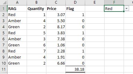
• Have a column of labels in column A, lets assume RAG status’
• Have a separate drop-down in cell F1 to select one of the label options (Red, Amber & Green)
• Values to be multiplied and summed in columns B & C
• Have a column alongside the data (column D) that checked the label and returned a 1 or 0 depending on it matching the drop-down:
  • =IF(A2=$F$1,1,0)
• Include this column within the SUMPRODUCT to only include the matching rows in your result.
  • =SUMPRODUCT(B2:B10,C2:C10,D2:D10)

Okay, so now we want to remove this helper column (D) and all the IF statements.
Here’s how:

• =SUMPRODUCT((A2:A10=$F$1)*(B2:B10)*(C2:C10))

What just happened there?

Right, it isn’t immediately obvious. First off we’re ignoring the ‘comma separated list of arguments’ structure that is normally used. Everything between the outer brackets becomes the only input the the SUMPRODUCT formula itself. This basically means that it’s only going to SUM the resulting input, but it still benefits from the array handling we mentioned earlier, and this is where the magic is happening.

The bracketed elements within the function are being multiplied together (* being a multiply symbol in this case). The second and third element are purely references to the values within columns B and C. Nothing exciting happening there. The first element however points to not a value column but the one we stored the RAG labels. This is obviously not something we can multiply by or sum. However, this array of labels is being compared to the label in the drop-down cell (F1). The equals within this element is asking the question:

“For each element in this array, does it match the thing on the other side of the ‘=’ sign?”

In our example this will return True for each RAG label that matches our drop-down selection and False for the rest. That’s great but these still aren’t numbers, we can’t math them; can we? Well, yes, as it happens, we can. If you perform any arithmetic function on an array of True and False values, Excel will convert them into 1’s and 0’s. There’s your binary flag!

Lookups

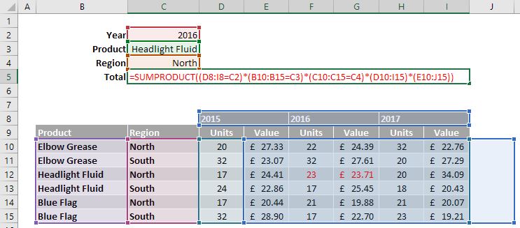
But we can go deeper still. There’s no need to involve any maths in the formula at all (kinda). Using these logical arguments you can use SUMPRODUCT to simply return a value you need. If you know that there is only one value in the data set that matches all the criteria (often when you want a specific value for a day/department etc.) then you can reference a single return array. This way all the logical tests return only one row that is one times the return array values and all the rest will be zero times. The formula will still add up all the values but there will be only the one. This can work with two dimensional arrays as easily as one.

Sure, you can use INDEX-MATCH or the like to do the same ting but SUMPRODUCT allows you to have multiple criteria on each dimension, easily parse your logical tests (especially when using named ranges and Tables). You can also perform a neat trick and offset your value arrays.

What is this “Offsetting of value arrays” you speak of?

I’ll need a picture to illustrate this one. The arrays being compared need to be of matching dimensions, i.e., the same number of entries for one dimensional arrays (lists), and matching lengths for each ‘side’ of a two dimensional array. However, they don’t need to be next to each other in the form of a table. That may not sound like that big a deal but it can come in very handy when managing irregular data sets. In one case I had a table that was set up with dates as column headers but two columns of data under each one. I was referencing from the top and sides of the table but the values taken from two 2D arrays, each offset by one cell. That’s a pain to do without SUMPRODUCT but this awesome function eats it up and spits out the answer without any fuss at all (see the image below for an illustration; of the range boundaries – not of the eating and spitting).

So that’s my case for SUMRODUCT being the star of the Excel function show. I’ll not deny there are some strong contenders but for me, this is the winner. No doubt this has a lot to do with the types of work I most often find myself doing. So do you have a favourite? Tell me, convince me, what can topple this king of Excel?